fT
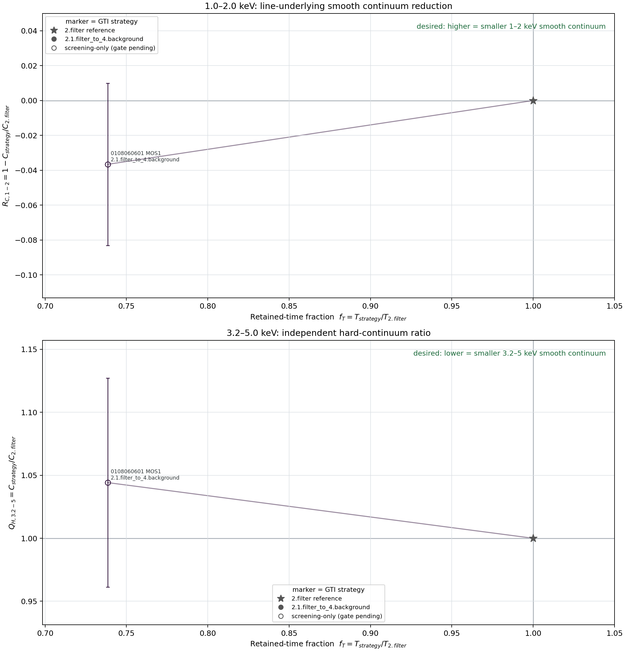
Tstrategy/T2.filter; this is a deterministic quantity once GTI is frozen, so no horizontal error bars are invented.
For the same ObsID × MOS, compare the time retained under different GTI strategies with two independent, response-folded, line-constrained continuum spectra.
Tstrategy/T2.filter; this is a deterministic quantity once GTI is frozen, so no horizontal error bars are invented.
1−Cstrategy/C2.filter. Above zero means the 1–2 keV continuum actually decreased.
Cstrategy/C2.filter. Below one means the 3.2–5 keV continuum actually decreased.
Not BPL norm, not raw PHA rate. Each value is the integral of all non-instrument-line components of the live XSherpa model under the same aperture, mask, XARTATOMS S/N+resolution grouping and respective ARF/RMF: LHB + absorbed halo + absorbed CXB + flat-response broken-SP. The Al/Si instrument lines are not counted in C.
The main figure is fixed at 1.0–2.0 keV, the smooth continuum under the Al/Si instrument lines; the lower figure is the independent 3.2–5.0 keV ratio. Vertical error bars come from the full Sherpa local covariance matrix propagated by live-model numerical differentiation, preserving the A/B0 correlations from shared sky parameters.
Colour indicates ObsID × MOS, markers indicate GTI strategy; same-colour thin lines connect to the common 2.filter reference point. Solid points are the formal Pareto points with all gates passed; open points are screening pilots only, explicitly retaining failed/incomplete gates and cannot be used to claim SP has been identified or a strategy has won.
0800730101 MOS2: 9 real GTI multi-strategy screening under the same 2.filter reference →
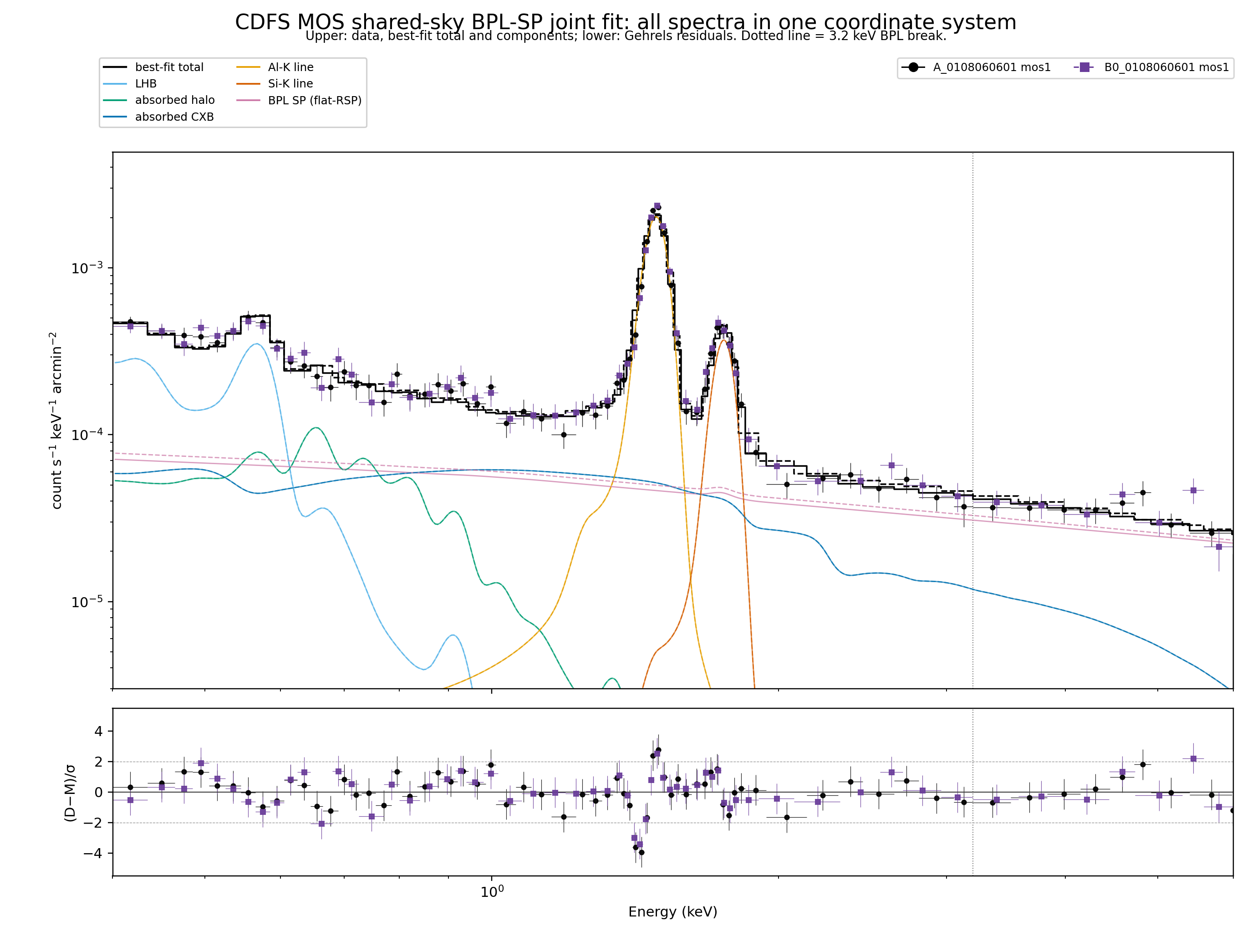
The same coordinate system overlays the A/B0 data, total model, all model components and Gehrels residuals; the BPL here is the flat-response detector-space term. It is the diagnostic figure for reading residuals, not a proxy back-derived from the line plot.
The table publishes only judgement-ready metrics; no event, GTI, PHA or response paths are released.
| case / strategy | level | fT | RC,1–2 ± 1σ | QH,3.2–5 ± 1σ | C1–2 (std → strategy) | gate |
|---|
Fixing the sky hypothesis makes the same pointing's sky cancel more cleanly across strategies, but does not by itself prove that the C difference is SP. Only after released-sky consistency, line-tie, response and residuals all pass do solid points enter the formal Pareto judgement. Stable, non-time-varying SP will not be removed by any GTI principle and still has to be handled in the spectral model.