Which "good times" are truly good?
A criterion-based definition of soft-proton contamination time filtering
Research plan for first-year graduate students in physics. No prior X-ray astronomy background is assumed. All tasks are implemented with public archive data and free software on a workstation.
Abstract
Space X-ray telescopes are contaminated by soft protons: low-energy particles from the Earth’s magnetosphere that the mirror focuses onto the detector. Because they are focused and produce a smooth continuum-like spectrum, soft protons and the sky cannot be distinguished by a single spectrum alone. The handle is temporal: soft protons arrive in bursts, so the standard practice is to drop whole noisy intervals.
That practice is based on a conventionally chosen threshold and no one has proved what that threshold should be. This project asks a sharper question than "which time bins are noisy": which timing cut minimizes what quantity? and then finds the cut that minimizes that quantity. The answer is based on two physical fingerprints that separate soft protons from the other background class, an explicit three-part error budget with different behaviors, and—crucially as shown in prior work—willingness to conclude either that the conventional threshold was already near optimal, or that it is throwing away good time.
1. Problem
1.1 What is measured, and why it is fragile
There is faint hot gas between stars and galaxies. It is too dim to be seen directly, but it emits in X-rays. Measuring this glow can tell us how much ordinary matter exists in the Universe, where it is, and how galaxies heat and expel their own gas.
This is a background measurement: you do not measure a bright source. You remove all bright components and then estimate the remaining diffuse, weak floor.
That makes the project unusually sensitive to "anything else that can produce faint diffuse signal", because such things can look like the target, not like a mistake.
1.2 Soft protons
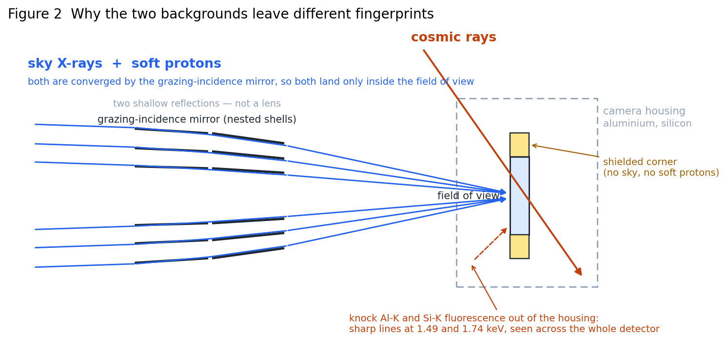
Protons with energies of tens to hundreds of keV are trapped and accelerated in the terrestrial magnetosphere. Incident-angle X-ray mirrors cannot separate them from photons: they are focused onto the detector along with the sky (Figure 2). In the detector they deposit energy in silicon and are recorded as events, creating a smooth continuum-like spectrum over the full band.
They are central in this field for two reasons:
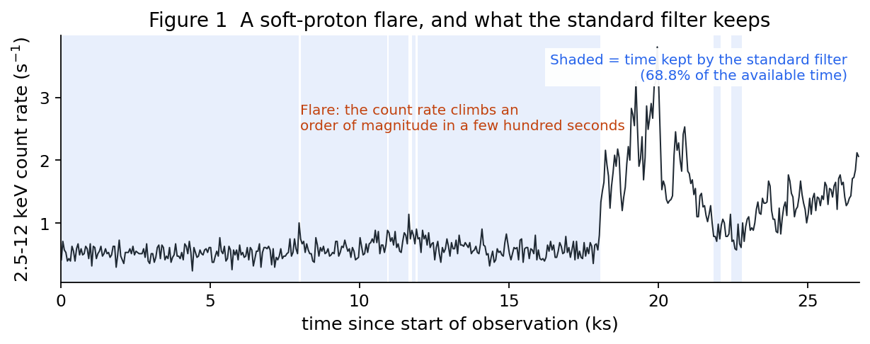
- They vary in time. Their amplitude can rise by an order of magnitude within minutes (Figure 1). Within one observation they can be almost absent or utterly dominant.
- They have no distinct spectral features. Their spectrum is smooth and lands exactly where diffuse sky emission is also observed. So a single spectrum in a single observation has no obvious identifying handle.
1.3 Another background, not the same thing
The detector also records cosmic-ray particles: high-energy particles traversing spacecraft and camera housing from all directions and not focused. They create their own continuum and sharp features: fluorescence lines from aluminum and silicon in the camera housing near 1.49 keV (Al-K) and 1.74 keV (Si-K).
Distinguishing these two is essential because only one type can be handled by GTI time cuts. If you time-cut the other type, you lose exposure for nothing.
2. Standard practice, and its hidden assumption
The standard treatment is called GTI (good-time interval) selection. You build a lightcurve in a high-energy band where the sky is dark and flares stand out, choose a threshold, and keep only times below threshold. All bins above threshold are dropped along with all celestial photons that arrived in those times.
This is sensible and effective. In the preliminary sample used previously, standard filtering removed 116.8 ks across 29 observations, and in 98.4% of those removed bins the rate is clearly noisier than the retained time. The method is not grossly wrong.
But three points have never been established:
- The threshold is conventional. It is not derived from a statement of what a final measurement should achieve.
- The cost is invisible. Dropping time increases the statistical uncertainty on the quantity you want to measure. In the pilot sample, standard filtering kept 68.8% useful time for one observation and only 30.2% for another. That is a large, unexamined penalty.
- There is no check for the most dangerous failure. A cut that removes real sky signal—for example a variable source inside the field of view—looks successful under standard criteria. Nothing catches that failure.
This project replaces convention with a criterion, and adds that missing alarm.
3. Theoretical basis: two fingerprints
This project stands on two properties of this instrument. Both are elementary, model-independent, and together turn an unanswerable question into an answerable one.
3.1 Geometry: soft protons never reach the shielded corner
The mirror focuses events into the field of view (FOV). A portion of the detector lies outside the FOV and is shielded from the sky, i.e. the unexposed corner. Sky photons do not reach there; soft protons also do not, because both follow the same focused paths. Cosmic rays arrive from all directions and do reach it.
So the corner is a direct, simultaneous, and sky-independent probe of only the particle background. Subtracting corner-count rate from an in-FOV count rate (after calibration) removes the cosmic-ray component and leaves sky plus soft proton—estimated on a per-observation basis. This is important because cosmic-ray background varies strongly across observations, while soft-proton fluctuations in this context are the target.
3.2 Spectra: soft protons carry no shell fluorescence line
Al-K and Si-K lines are produced when particles strike the camera housing. Soft protons are focused through the mirror and deposit energy directly in silicon, so they do not generate these lines. Cosmic-ray background produces both continuum and both lines with a fixed ratio.
Therefore, the removed-component line-to-continuum ratio gives a label. No spectral model is needed: we compare two subsets from the same data, same detector, with the same model inputs.
4. Preliminary findings
Preliminary work covers 30 archival observations in the M31 outskirts. They were chosen because they are large and homogeneous and have strong flare variation—some are nearly clean, some exceed 80% flare-flagged exposure. Three findings emerged.
4.1 The removed intervals are not cosmic-ray background
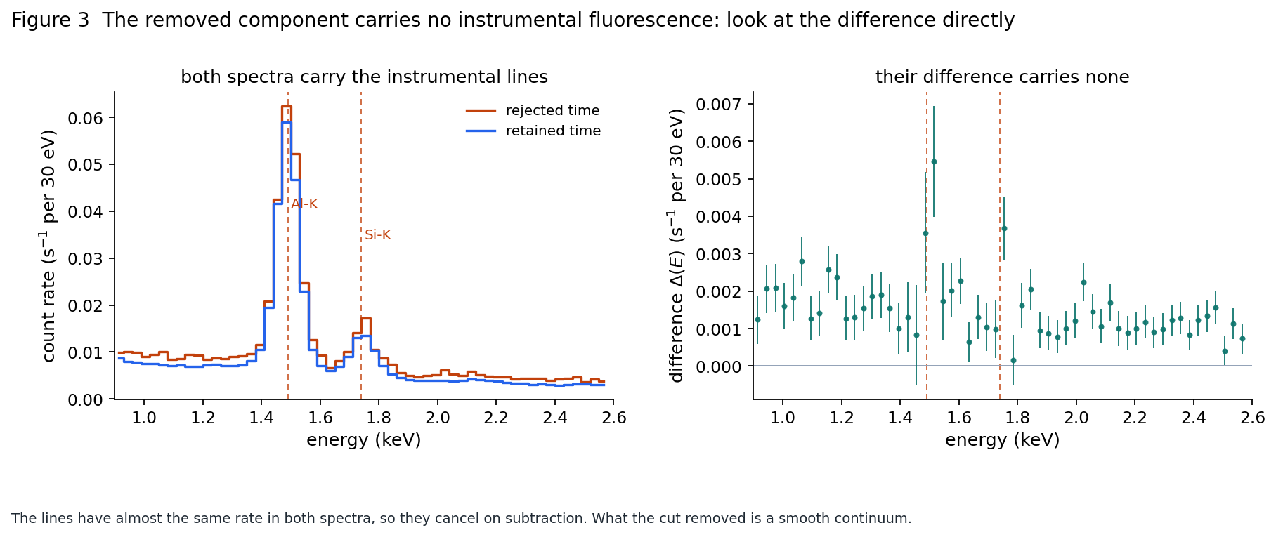
Figure 3 compares two spectra and their difference directly. Both removed and retained spectra include Al-K and Si-K lines—important, because both time subsets share the same particle background. In their difference, the lines almost vanish.
This mechanism deserves a careful explanation because it is easy to misread. Define:
where \(R_{\rm rej}\) and \(R_{\rm ret}\) are count-rate spectra of rejected and retained bins. Fluorescence lines are caused by particle hits in camera housing, and if their count rate is the same in both subsets, they cancel exactly under subtraction. They are not being "subtracted too much"; they are simply absent in the difference. The remaining \(\Delta(E)\) is a smooth continuum—the shape expected for soft protons.
(A common misread comes from plotting the normalized excess \(\Delta(E)/R_{\rm ret}(E)\). At the Al lines, the denominator is lifted by the line while the numerator is not, so the ratio dips. That dip is a ratio effect; the physical content is still "no line in \(\Delta\)".)
But "same line rate" is an assumption, and it is directly testable. Splitting each observation into quiet and flare intervals, the continuum rose by +442% while the Al-K line changed by only +0.35% (Figure 8). This is the hard basis for the proposal: the fluorescence line is an internal, in-FOV particle monitor proving that the linearly varying component is not changed by flare periods. The method and its caveats are in §8.2.
If removed time only contained more cosmic-ray background, both lines should rise proportionally with continuum. They do not.
4.2 It also does not reach the shielded corner, and it is not a source
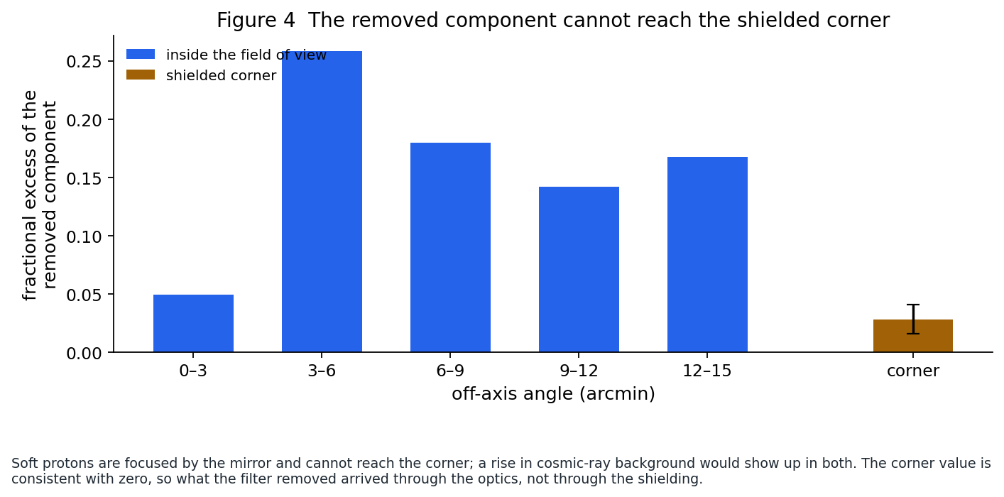
Figure 4 measures the same removed component inside the FOV and in the corner. Inside the FOV it is 14–26% of the count rate; in the corner only 2.8%, statistically consistent with zero. This removed component is therefore mirror-focused.
But "mirror-focused arrival" leaves one remaining possibility—and it is severe: a variable source inside the field. A variable star or X-ray binary also arrives through the mirror, also carries no shell fluorescence lines, and also varies in time. If such a source is cut, then real sky signal is removed, and by current standards every criterion reads as "successful".
The distinction needs spatial information, but does not require source detection. The criterion uses the removed component's own spatial distribution: split the FOV grid and compare the brightest-cell share to the diffuse baseline \(1/N_{\rm cell}\).
- Point source: regardless of grid size, it packs a large fraction into a single cell—tens of times above the diffuse baseline, and the ratio increases as grid cells get smaller.
- Diffuse component: stays near baseline across grids; the ratio is approximately constant.
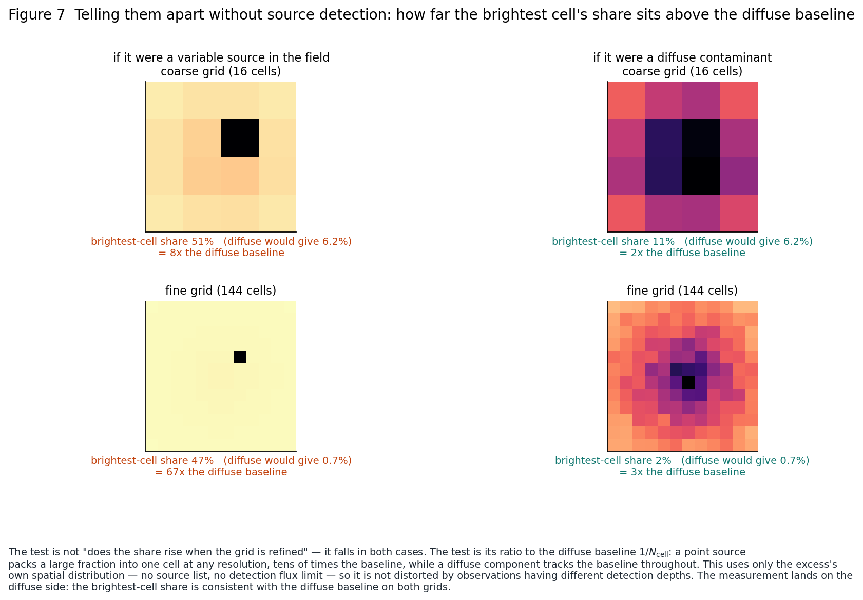
One practical advantage is worth emphasizing: this is independent of source catalogs and detection throughput. Detection depth depends on exposure; since we will alter exposure by GTI choices, using a source catalog introduces a self-referential systematic. Looking only at the distribution of removed excess avoids this feedback.
Measured results support a diffuse origin: in both coarse and fine grids, the brightest-cell share is consistent with diffuse expectations and does not increase when grids are refined. Point-source interpretation is excluded.
4.3 Trade-offs are worse than expected
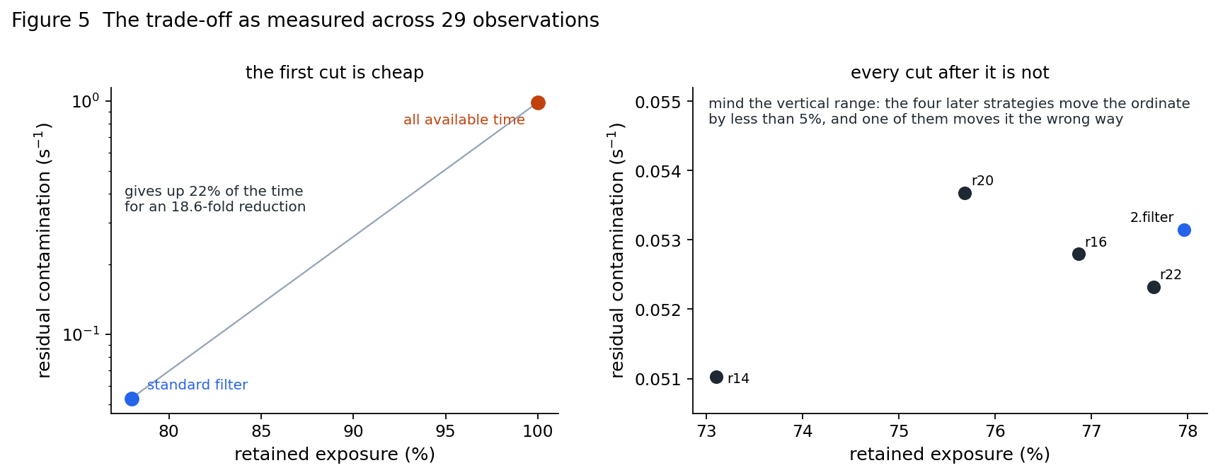
Figure 5 puts retained exposure against a residual contamination proxy for the full sample. Standard filtering removes 22% useful time and reduces the proxy by 18.6×—an excellent trade. On top of that, four progressively more elaborate strategies move the same proxy by less than 5%, and one of those moves it in the wrong direction, all while losing exposure.
I need to make one point explicitly because it directly motivated this proposal. The y-axis in Figure 5 is
where \(K\) is the selected retained time set, \(T(K)\) is the \(K\) total live time in seconds, and \(N_{\rm FOV}(K)\) and \(N_{\rm corner}(K)\) are event counts in FOV and corner within \(K\). This y-axis is imperfect: \(\alpha\) was calibrated with an origin-forced regression, which pulls true sky into \(\alpha\), overestimates by >1×, and amplifies particle-background fluctuations into the y-axis with sign flip (detailed in §8.2). The misdirected strategy in that plot is the strategy that depends most strongly on this axis.
So this proposal does not patch that y-axis; it replaces it with the quantity defined in §8.1 that needs no particle-background normalization. But the qualitative conclusion is unchanged: standard filtering removes most of it, and later strategies merely contest the remainder. Recomputing with the replacement quantity strengthens this conclusion: standard filtering has median removed efficiency 0.990, meaning all remaining strategies are competing within roughly 1%.
This observation created the proposal. The field has been optimizing in a regime with steeply diminishing returns, while lacking any criterion that can tell us this.
5. Research questions
There are two questions, not one. They look almost identical in wording but optimize different error budgets.
Q-single. Given one complete observation, which time intervals should be kept to produce the most accurate measurement of the diffuse sky?
Q-multi. Given many observations, which time intervals should be kept in each observation to produce the most accurate measurement of the diffuse sky?
In one observation, statistical error dominates: trimming time directly raises it. The trade is "less contamination" versus "less counts", both computed within that single observation.
In many observations, statistical error keeps decreasing with exposure while observation-to-observation biases do not—that is systematic error, and this proposal is built to handle it. §8.6 gives an explicit result: the two optimizers are not at the same point, and the number of observations \(N\) is the control knob that shifts the optimum from one to the other.
Important distinction:
QPB inconsistencies are usually explainable. For each observation, mos-back provides its own QPB estimate and subtraction, so that contribution can be propagated. Soft protons are not handled. They lack a corresponding model product, and that is the irreducible cross-observation bias this project addresses.
So three sub-questions:
- Q1. What is the right quantity to minimize, and what is its explicit single- and multi-observation form? Can it be measured from the data themselves, rather than assumed?
- Q2. Where does conventional filtering lie relative to that optimum—is it at, before, or beyond the minimum?
- Q3. Does removing more contamination actually make repeated observations of the same sky more consistent? This has not been tested before, and current methods quietly assume it.
6. What "better" means: error budget
This is the core concept and must be precise, because the standard approach is weakest exactly here.
6.1 Single observation
After subtracting the corner monitor from §3.1, sky surface brightness from one observation has a familiar statistical term:
where \(T\) is retained live time. So trimming time increases this term by \(1/\sqrt{f}-1\) if retained fraction is \(f\). For example, keeping 89% raises the statistical term by 6%.
What trimming gains is a reduction in the second term: the residual variable soft-proton contamination in kept time, \(b\). This is bias, not noise—adding counts does not reduce it. Total MSE for one observation is
Minimizing \(\mathcal{E}\) over "which intervals to keep" is a well-defined problem with a unique solution, and it naturally stops where the residual term is flat and further cuts only increase the first term.
6.2 Multiple observations
The rationale for combining observations is lower uncertainty, but the three terms shrink differently. This is the key structural fact of this proposal (Figure 6):
| Contribution | Behavior when combining \(N\) observations |
|---|---|
| statistical error | decreases as \(1/\sqrt{\sum_i T_i}\); more total exposure always helps |
| between-observation varying contamination | decreases as \(s/\sqrt{N}\)—averaging helps; \(s\) is the spread of residual contamination \(b_i\), where \(s^2=\mathrm{Var}(b_i)\) |
| contamination identical across all observations | does not decrease at all |
Time filtering can affect only the second row: contamination with no time structure cannot be moved by any GTI rule.
The third row is invisible in the data—adding the same amount to each observation is indistinguishable from intrinsic sky brightness. To constrain it one must do proper spectral fitting: include residual soft-proton with its own spectral shape in a joint model and separate it from the sky component via spectral mismatch. That is outside this proposal’s scope, but we must state this boundary—otherwise readers infer time filtering solves everything.
For combined estimates weighted by \(w_i\):
This immediately yields two practical conclusions, both absent from current practice.
Consistency is necessary but not sufficient. Soft protons only increase counts, so it is the weighted mean of bias, not its spread, that hurts combined results. If contamination levels are identical, observations appear perfectly consistent and jointly biased. Between-observation consistency is a detector symptom, not the target measurement.
Time cuts are not the only lever. Weights \(w_i\) are free parameters. An observation with high stable contamination cannot be improved by time cuts (no time structure), but it can be down-weighted and this does not lose exposure. A framework based only on time cuts does not see this option.
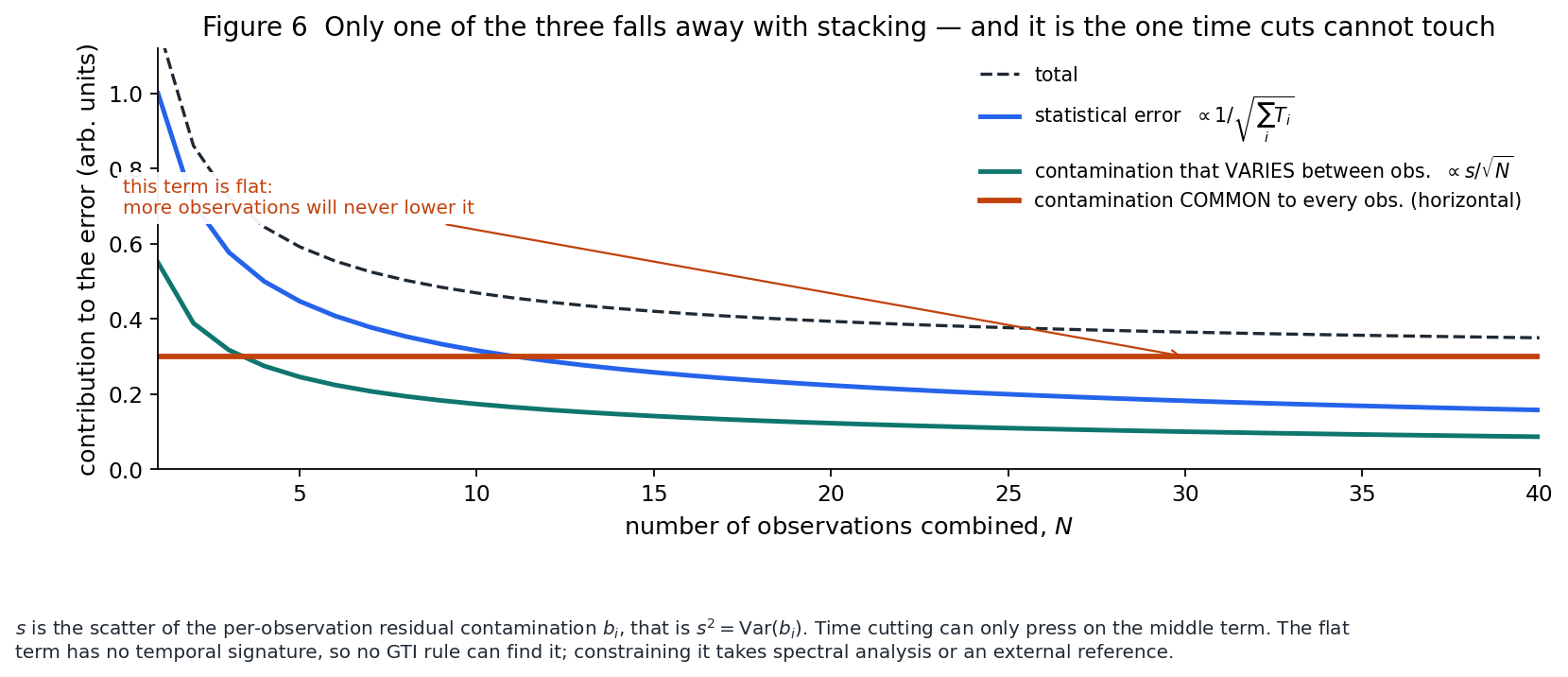
In Figure 6, the first two terms fall with \(N\), with different rates; the third is a flat line and is fully unremovable by any GTI rule.
7. Materials
Data. Archival XMM-Newton ODFs are publicly available for every observation used. This proposal uses MOS2 data from 30 outer-M31 observations 080073*01 in preliminary work; the same method applies to any set with mixed "clean and flare-contaminated" and repeated or nearby pointings.
Software. ESA SAS and its ESAS package produce spectra and responses from ODFs. Exploration of GTI strategies occurs before or inside the 2.filter stage of the pipeline and is simple array logic; it does not require rerunning ESAS for each trial, which keeps iteration cost low.
Three required inputs, all necessary. (1) Full-event tables: EMCHAIN output before any flare screening. Archive products typically contain pre-filtered event lists and cannot test whether "we could keep more." (2) 1 s FOV and corner lightcurves, covering the entire interval. (3) A one-pass CCD pre-clean: run SAS emanom to remove CCDs entering anomalous state; those CCDs show soft, line-free local excess that can pass both §8.2 checks.
8. Methods and definitions
This section is core to proposal review. Each quantity has a definition, its physical dependence, its uncertainty source, and when it can fail.
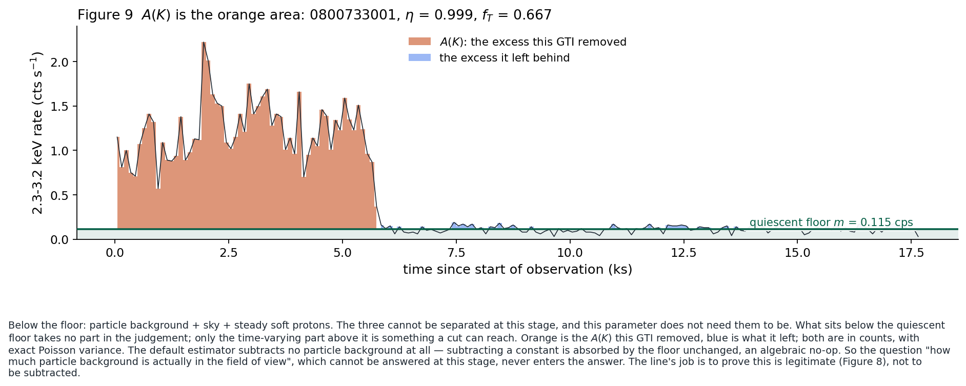
8.1 Core quantity: how much variable soft-proton excess this GTI removes
First, the notation is fixed. Divide the full observation into equal-length bins; bin \(j\) has length \(\tau_j\) (set to 100 s here). \(c_j\) is the count in 2.30–3.20 keV for that bin. This band is chosen because it has no instrumental fluorescence lines and sits below the soft-proton broken-power-law break at 3.2 keV, where the spectrum is harder and therefore the soft-proton fraction per count is larger while particle-background fraction is smaller (§8.3). Define
where \(m\) is the quiet baseline, the weighted average of bins around the mode of the observation's count-rate distribution (methods and why iterative σ-clipping is rejected are in §8.7). For any candidate GTI \(K\):
- \(A(K)\) is the excess above baseline rejected by GTI \(K\), in counts. Its count variance is exact Poisson; \(m\) is estimated and not propagated in this expression, which underestimates its uncertainty by about 4% median (28% worst-case), so this should be added.
- \(A_{\rm tot}\) depends only on observation and \(m\), not on \(K\)—that is why it can appear in the denominator.
- \(\eta(K)\) is removal efficiency, nominally in \([0,1]\). But because both numerator and denominator are noisy, retained intervals can produce negative residual excess in kept time and \(\eta\) can dip slightly above one. That offset is itself a diagnostic: it should match noise expectations, and if it does not, the baseline was probably misestimated.
The scope must be explicit, or this quantity gets misread. \(A_{\rm tot}\) is not "how much variable soft proton is physically present". That is not observable directly here. It is "excess above the baseline we define." Equating the two turns a construction into fact.
The accurate statement is model-based. Let \(c_j=(\,\mathrm{sky}+\mathrm{QPB}+SP_j)\,\tau_j\) and \(m=\mathrm{sky}+\mathrm{QPB}+SP_{\rm floor}\), where \(SP_{\rm floor}\) is the soft-proton level in bins judged quiet. Then
This equation is exact only if sky and particle background are constant over time; the second condition is measured (§8.2, lines are stable during flares at the 0.35% level), while the first is an assumption. The spatial test in §4.2 excludes source variability, but this is exclusion, not proof.
From this come three boundary statements and a direct limit on what the quantity can claim:
- \(A_{\rm tot}\) is the number of soft-proton counts above our chosen quiet baseline. The true minimum in the same observation can be lower than \(SP_{\rm floor}\), so it is a lower bound, not the truth.
- Hence \(\eta\) is not "percent of soft protons removed." It is "percent of the defined excess removed."
- Its defensible use is: within the same observation and fixed \(m\), compare different GTIs—the unknown part cancels exactly in comparison. Across observations, \(\eta\) already depends on how \(m\) is defined, so include the systematic baseline uncertainty from §8.7.
To turn the lower bound into a truth estimate, there is only one route, and it is not in the time domain. If one observation is nearly proton-free, that baseline gives \(\mathrm{sky}+\mathrm{QPB}\), so differences \(m_i-m_0\) among observations become each observation's stable soft-proton excess. That moves from "unobservable" to "measurable relative to cleanest sample." To get absolute values requires spectroscopy: the 3.2 keV break measured in §8.3 gives a soft-proton spectral template, and sky is not a broken power law, so joint fitting can in principle separate that baseline component. This proposal does not execute that step, but states explicitly where the boundary is.
Why this definition is stronger than legacy y-axes. \(\eta\) uses only this observation and this candidate \(K\); it does not reference a different strategy. So it is legal to compare across strategies with different kept time. Any ratio-form "compared to a reference" does not have this property—the denominator changes with cut depth, so the same physical component can flip a decision as cuts vary.
What lies below the baseline is not in the decision, and that is its power. \(m\) contains particle background, sky, and irreducible stable soft protons. These are inseparable in 2.filter without mos-back and current data alone (\(\alpha\) needs calibration as in §8.2). The parameter does not require their decomposition: it only concerns the time-variable component above baseline. Figure 9 draws this construction for one real observation.
Measured results. Taking \(K\) as the archived standard 2.filter GTI for 30 observations:
| \(A_{\rm tot}\) is significant (\(\ge5\sigma\)), so \(\eta\) is defined | 19 / 30 |
| Median \(\eta\) for these observations | 0.990 |
| Retained-time fraction \(f_T\) | Median 0.690 |
| Removed excess above baseline in full sample | 136516 counts |
Changing the energy band does not alter the conclusion, and it is measured. Above the break (3.20–4.50 keV), median η is 0.998; across the break (2.30–4.50 keV), 0.991; in soft band (0.50–1.30 keV), 0.979; median per-observation differences 0.0068. \(A(K)\) is a count statistic and is not by design very sensitive to band, but this had to be shown.
Standard filtering drops a median 31% of time for \(\eta\approx0.99\)—about 1% residual excess above baseline. This turns the "diminishing returns" intuition of §4.3 into numbers: the subsequent more elaborate strategies are competing over roughly the last one to two percent.
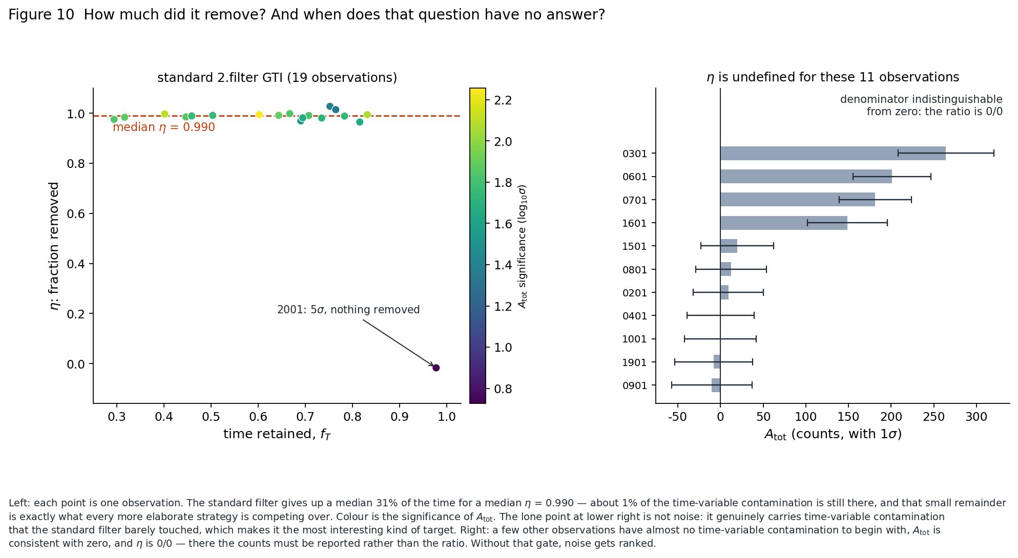
It must be said when this fails. \(\eta\) is a ratio and becomes \(0/0\) if \(A_{\rm tot}\to0\). In the sample, 11 observations are excess-consistent with zero; for these, one should report \(A(K)\) counts and not \(\eta\), otherwise noise gets sorted as signal. This is not corner-case: those 11 are over one-third of the sample.
8.2 Fluorescence lines: in-FOV particle monitor, and why corner alone is insufficient
\(A(K)\) is defined with no particle-background subtraction. This needs justification, and that justification is measured, not assumed.
First, why the corner alone is insufficient. The corner sees particle background only. To convert corner count rate to FOV particle rate requires transfer coefficient \(\alpha\), and 2.filter has no mos-back. In early work we estimated \(\alpha\) from scientific data alone: in the quietest bins we enforce FOV excess zero, i.e. \(\alpha=\sum N_{\rm FOV}/\sum N_{\rm corner}\), forcing the fit through the origin. This is wrong, and the error is quantifiable: the FOV contains sky while the corner does not, so forcing the origin puts sky fully into \(\alpha\). Regression on static levels across 30 observations (intercept absorbs sky) gives:
| Origin-forced \(\alpha\) | 4.28 |
| Regression slope \(\alpha\) | 1.93 ± 0.53 (bootstrap [1.57, 2.54]) |
| \(P(\text{slope}\ge4.28)\) | 0.0014 |
\(\alpha\) is too high by more than 2×. The consequence is that corner rate in the sample shifts from 0.113 to 0.165 cps, so \(R_{\rm FOV}-\alpha R_{\rm corner}\) adds \((4.28-1.93)\times0.052=0.122\) cps as spurious excess, while the stable FOV rate is only 0.614 cps. Direction is wrong: higher particle background makes GTI look cleaner. In trying to guard against QPB variation, this corner monitor amplifies QPB variation by about 2× into the same metric.
Hence this proposal does not subtract using the corner. A valid use remains: the corner is an independent, fast particle-variation probe to validate "particle background changes slowly." It is a validator, not a subtractor.
The true in-FOV monitor is inside the FOV. Aluminum and silicon K fluorescence from cosmic-ray impacts in the camera housing follows particle variation and is not produced by soft protons. It is measured in the same aperture and readout as your sky data, with zero transfer coefficient. So we can directly test the key assumption: does background vary during flares?
Using full-event tables to split each observation into quiet and flare intervals, measurement gives (Figure 8):
| Quantity | Flare / quiet median across sample |
|---|---|
| Continuum (2.3–3.2 keV) | +442% |
| Al-K line (log-parabola + Gaussian fit) | +0.35% |
Threefold increase in continuum, line stable. Therefore subtracting no particle term in \(A(K)\) is justified: particle background is constant during flares and sits in the baseline \(m\). Subtracting a constant is absorbed in \(m\) and is an algebraic no-op.
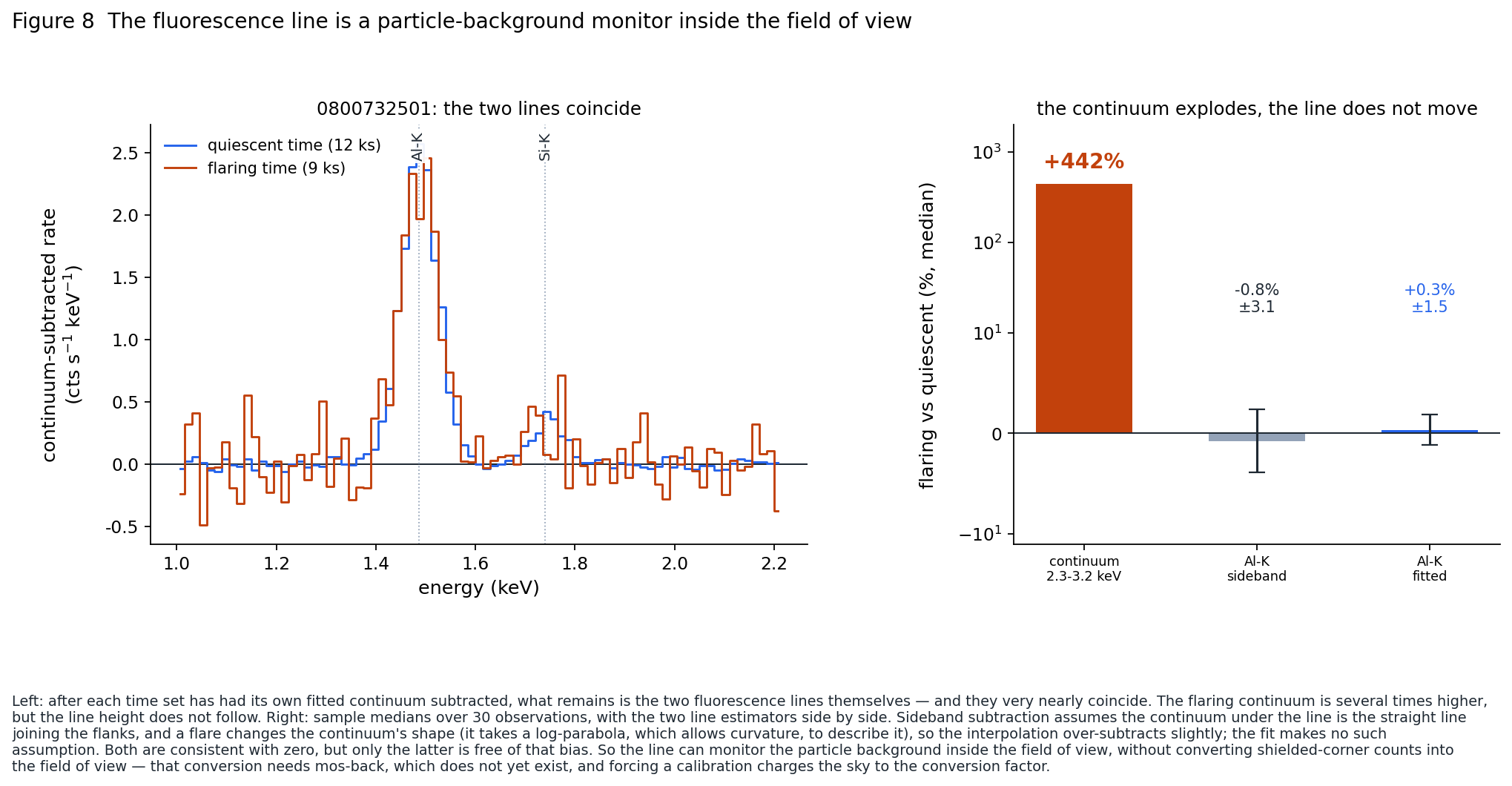
There is a methodological lesson here, and it is more surprising than initially expected. Line strength can be measured two ways: side-band subtraction, assuming line wings interpolate linearly, or fitting, jointly fitting continuum and Gaussian line. These methods gave -0.76% and +0.35% in this sample, both consistent with zero, but side-band subtraction carries a known directional bias because flares change the shape under the line and invalidate linear interpolation.
The used fits model the continuum as a log-parabola. It deserves explicit context as the only model assumption in this section:
In log-log space, a power law is a line; a log-parabola adds one curvature term \(\beta\), becoming a parabola. With \(\beta=0\) it reduces to power law, so the model classes are nested and can be compared via likelihood-ratio test rather than visual residual inspection.
It is not a physical model of the source, only a local interpolation under the line. The only requirement is smooth curvature on scales much larger than the line width (fit \(\sigma\approx39\) eV), so line photons are not absorbed.
The hypothesis test reverses one intuition. \(2(C_{\rm PL}-C_{\rm LP})\) follows χ² with one degree of freedom for the null \(\beta=0\) (3.84 at 95%, 6.63 at 99%):
| Spectrum | Median \(\Delta C\) | \(>95\%\) | \(>99\%\) |
|---|---|---|---|
| quiet intervals | 9.1 | 20/23 | 17/23 |
| flare intervals | 2.9 | 6/23 | 2/23 |
Curvature is required in quiet spectra, not in flare spectra. This is interpretable: quiet spectra are sky-dominated and contain Fe-L + Mg XI line complexes plus the 1.84 keV Si K edge in the 1.0–2.2 keV region; flare spectra are proton-dominated, where a broken power law is expected to be a harder law below 3.2 keV (§8.3). So "flare spectra look more power-law-like" is independent confirmation of the expected SP fingerprint.
Systematics from model choice were measured too. Replacing continuum with pure power law changes line variation from +0.35% to +0.64%, a shift of 0.29 percentage points; the statistical uncertainty on this ratio is about 1.5 percentage points. The common-mode shift mostly cancels in the flare-vs-quiet ratio, so line model is not the dominant systematics here, but must be reported because it is on the same order as the signal.
One final point: I previously reversed a causal direction. The earlier method's side-band over-subtraction was misread as "particle background decreases with time"; in 30 observations this occurred in 13 cases. Using the corrected quiet definition and fitting reduces this to 10, but it still remains a systematics row (§8.7).
This has immediate consequences for existing workflow. The prior 2.1.filter/2.1c method constructs symmetric high/low tests on a wide detector-rate axis and uses Al-K as the common instrumental line constraint shared by the two arms, then independently fits continua and takes \(C_{\rm high}-C_{\rm low}\) as the candidate variable component spectrum. That "line is shared" constraint used to be a working assumption and was not tested. Now it is measured and can be converted into tolerance: line mismatch upper bound (at \(2\sigma\)) is 3.4%, static line rate is 0.203 cps, and continuum contrast is 0.51 cps, so forcing line consistency biases continuum by at most
And this test used +442% continuum contrast, stronger than the symmetric high/low contrast in practical use, so the bound is conservative.
8.3 Identity of the removed component: why it supports metric validity
\(\eta\) states how much excess above baseline is removed. It does not claim that excess is soft protons. To use \(\eta\) as "contamination removal efficiency", the removed component must independently be established as contamination. This section provides three independent pieces; the first two exclude alternatives, the third is positive.
Start with the third because it is strongest. The residual SP spectrum is conventionally represented by a broken power law with a break near 3.2 keV, and a harder index below the break. This is a falsifiable prediction: if the removed component is soft protons, the stacked difference spectrum (flare minus quiet, in count space) should steepen above 3.2 keV. Measured in all sample observations:
| Below 3.2 keV | Above 3.2 keV | Steepening amount | |
|---|---|---|---|
| Removed component | \(+0.698\pm0.018\) | \(+1.074\pm0.007\) | \mathbf{+0.376\pm0.019} |
| Quiet spectrum (same response, different source) | \(+0.889\pm0.032\) | \(+0.318\pm0.009\) | \(-0.571\pm0.034\) |
Directions are opposite; difference is \(+0.947\pm0.039\), i.e. \(24.4\sigma\). This control is needed: the gold M edge sits in 2.2–3.5 keV and could induce spectral curvature there. Response effects are shared by both spectra, yet the directions differ in opposite signs; therefore this steepening is an intrinsic property of the removed component.
This is stronger than "no lines." Not carrying fluorescence lines excludes one class of contaminant; break behavior is a positive prediction from soft-proton physics that is confirmed in data. It also supplies the spectral template mentioned at the end of §8.1.
Boundary. These are count-space measurements with no ARF/RMF and no unfolding, so values in this table are not spectral indices; break magnitude cannot be compared directly to literature broken-power-law parameters. What is robust is presence, location, and sign of the break, plus the quiet-spectrum contrast. To obtain physically calibrated photon indices, response matrices are needed, which is a separate step outside this proposal.
The other two pieces are on the same difference spectrum. For any candidate GTI, construct the excess
where \(n_{\rm rej}\), \(n_{\rm ret}\) are counts near energy \(E\), and \(T_{\rm rej}\), \(T_{\rm ret}\) live times in removed and retained intervals. The two sets are disjoint, giving exact Poisson variance; any component constant in time (sky, stable particle background) cancels exactly.
The other two are exclusionary: line/continuum ratio (§4.1, §8.2) excludes "removed is extra cosmic-ray background"; spatial compactness (§4.2) excludes "removed is a variable source in the field."
This is not just a pass/fail gate. In the objective, "removed continuum" is called gain, and that is valid only if the removed part is contamination. If part of it were true sky signal, that part should be counted as a second cost. These two measurements are therefore the basis for metric validity—without them, \(\mathcal{E}^2=\sigma^2+b^2\) has no defined \(b\).
Statistics are chosen linear in counts because this enables a null calibration. Linear loss metrics have a clean null distribution; line/continuum ratio is ratio-of-two-small-numbers with a pathologic null, so it is not usable for significance.
Known failure modes are listed here, not left for later interrogation. A CCD entering anomalous state mid-observation can generate soft-looking, line-free localized excess: in the line test it perfectly mimics soft protons, and in compactness it fills a single CCD while remaining near diffuse baseline on 20″/80″ grids. Both gates pass it. This proposal does not rely on metric detection for this; it is screened out before GTI strategy with SAS emanom per CCD—this is preprocessing work, not a burden for the objective itself.
8.4 Single-observation objective function
Inside one observation there are only two layers: a time-varying term and a constant term. The distinction between "observation-level constant above sample floor" and "identical across observations" is a sample-level construction: they are the same constant within one observation and are unmeasurable because they are degenerate with the sky.
Thus the honest statement is: one observation cannot define its own zero. The objective function for a single observation is well-defined only after specifying the zero, which must come from outside.
Given a zero, with \(f\) retained live-time fraction, \(T\) retained live time, and residual contamination \(b\) in retained time:
\(\mathcal{E}^2\) is variance + squared bias; therefore the sum of squares is principled. \(b(f)\) grows with \(f\) (more kept time brings more contamination), and \(\sigma^2\) falls with \(f\), so the internal optimum is unique.
How solved. Sort all full-time bins by \(p_j\) (§8.1) in ascending order and recompute \(\mathcal{E}\) after adding each bin. The curve vs retained exposure has a minimum; that is the answer for that observation.
The unmeasurable constant is not removed from optimization. Bias enters squared, and cross-terms keep it in the gradient: if the constant baseline is larger, cutting more is preferable. The practical method is to scan it as a parameter: zero is a conservative minimum-cut default; then report how the optimum shifts as it increases. Conclusions no longer depend on an unmeasured constant, while dependence is quantified.
8.5 Multiple-observation objective function
With \(N\) observations each producing sky brightness estimate \(x_i=SB+b_i+\text{noise}\), statistical error \(\sigma_i\), and one-sided bias \(b_i\ge0\), the weighted combination is
Minimize over both kept sets \(\{K_i\}\) and weights \(\{w_i\}\).
Two observations suffice for the full lesson. Let A be clean (\(b=0\)), B be biased by \(b\), both with statistical error \(\sigma\), and let B have weight \(w\) (A has weight 1). Closed form minimizer:
Three immediate results:
- The common "safe" approximation \(w_i\propto1/(\sigma_i^2+b_i^2)\) is exact here.
- \(\mathcal{E}^2_{\min}\le\sigma^2\) always. So an optimal weighted combination never gets worse by including a biased observation—the correct move is down-weighting, not dropping.
- If equal weights are used (simple \(w=1\)), adding B is useful only when \(b<\sqrt2\,\sigma\). This is the quantitative version of "consistency is necessary but insufficient."
With \(N\) observations, the new term is only that the bias is a weighted mean then squared, so observations are coupled in the gradient and the stationarity includes \(B=\sum_j u_jb_j\) where \(u_i=w_i/\sum w\):
When \(b_i\) is large, \(u_i\) is driven to zero—this is formally "discard that observation." That operation is already done manually in practice, but without an explicit criterion.
What "down-weight" means operationally. This is important because the standard chain has no such control. Once spectra are merged, they are weighted by exposure and cannot be undone. So down-weighting happens at the parameter level:
- fit each observation independently to obtain \(SB_i\pm\sigma_i\);
- combine with \(w_i\propto1/(\sigma_i^2+b_i^2)\) instead of default \(w_i\propto1/\sigma_i^2\) (approximately exposure).
The real operational cost is one: do not combine spectra before fitting.
Consistency is necessary, not sufficient. Bias has one sign, and what harms combined results is the weighted mean of bias. A set of observations with equal contamination are perfectly consistent and jointly wrong. Consistency is detector-level, not target-level.
8.6 Pareto: single-observation minima and multi-observation platform start
A Pareto frontier is not a flaw; it is a boundary of feasible solutions. The flaw is interpreting frontier points as evidence. Constrained optimization does not remove frontiers; it selects one point on them—and which one depends on whether Q-single or Q-multi is the task.
For \(N\) homogeneous observations weighted equally, retained fraction \(f\), \(\sigma^2_{\rm comb}=k/(Nf)\), residual contamination \(b(f)\):
- \(N=1\): solution \(2bb'=k/f^2\), both terms positive; optimum lies inside the frontier. On the platform \(b'=0\), derivative is purely negative, so we still cut further. Single-observation optimum keeps more time than platform start.
- \(N\to\infty\): first term goes to zero and root tends to \(b'(f)=0\), the platform start.
So \(N\) moves the optimum from one end to the other: more observations imply more cutting, because exposure is cheap and bias is the only enemy. The minimal point on the Pareto frontier belongs to the single-observation objective; platform start is the multi-observation constraint. They generally do not coincide, and their separation is an observable quantity.
New frontier points are no longer evidence. In preliminary work, a strategy highly effective on the observation where designed split positive and negative equally across 29 additional observations; high variance in y-axis and low variance in x-axis produced an envelope-chasing behavior. Only the strategy frozen on one sample and applied to independent observations is interpretable.
8.7 Unfinished choices and known-systematics price list
List them honestly, because they affect conclusions.
Baseline estimation method for \(m\). This is critical. Iterative σ clipping has two failure modes, both hit here: if the clipping threshold uses the estimated level, it collapses to a shrinking subset; if it uses fixed Poisson width on raw counts, \(3\sigma\) at 100 s is more than half the static rate, and flare shoulders survive, lifting the baseline. We therefore use a half-sample mode of the rate distribution peak, plus averaging within \(3\sigma_{\rm Poisson}\) on both sides. The mode is density-defined, so the tail cannot pull it and there is no collapse. Cost: median change in \(\eta\) between baseline methods is 0.0032.
Other choices and known systematics:
| Item | Current choice | Impact on \(\eta\) |
|---|---|---|
| Baseline definition (mode vs σ-clipping) | half-sample mode | 0.0134 (median) |
| Continuum band (below break vs across break) | 2.30–3.20 keV | 0.0068 (median) |
| particle-background drift (line linear term) | 10/30 observations \(>2\sigma\) | 0.0067 (median) |
| Constant anchor (should be zero algebraically) | max 0.046 measured | result of tie mode and non-zero overlap |
| below-line continuum model (power law vs log-parabola) | log-parabola | no direct impact on \(\eta\); 0.29 pp impact on line test |
| Time bin length 100 s | inherited from existing workflow | not yet measured |
| Significance gate for \(A_{\rm tot}\): \(5\sigma\) | pre-declared | determines whether \(\eta\) can be reported |
| How much stable soft proton sits in the baseline | unmeasurable | determines whether \(A_{\rm tot}\) is a lower bound or truth (§8.1) |
| Does the sky model include radial smoothness with source distance from the center? | 30 fields spanning 44.7′–134.8′ | coefficient should carry uncertainty, not be assumed |
| cosmic variance floor | different fields sample different unresolved sources | must be estimated, not assumed |
9. What would count as success, and what would falsify it
An impossible proposal is not a proposal. Clean outcomes are:
| Outcome | Meaning |
|---|---|
| optimum near conventional filtering | conventional practice receives quantitative justification. Useful: a short paper. |
| optimum keeps clearly more time | This field has been discarding good exposure. Direct benefit to users of this instrument family. |
| optimum keeps clearly less time | Residual contamination is larger than assumed; published background measurements carry unrecognized bias. |
| removed component carries fluorescence lines | proposal assumption fails for this sample; what is cut is cosmic-ray background. Report and stop. |
| inter-observation diffuse measurements do not change with cuts | Detector proxies are not tracking the science target. This would overturn common practice and is the most important possible outcome. |
Note the last two are hypothesis failure but project success. The phase-2 and phase-4 design ensures these are detected early, not after years.
10. Risks and mitigation
Invisible baseline. A contamination component identical across observations is fundamentally unobservable internally. That is a genuine, permanent limitation, not a bug. We report results as functions of assumed baseline values and use zero baseline as conservative default; this default understates any gain from cuts, so any demonstrated gain is not an artifact of that assumption.
Sources. A variable source in the aperture can perfectly mimic contamination in time. This proposal does not add a full frozen-source mask stack because that would introduce a circular dependency: changing cuts changes exposure, which changes detection depth, which changes masks. Instead we use the source-catalog-free spatial criterion from §4.2: examine spatial distribution of removed component only, and compare the brightest-cell share against the diffuse baseline. In the sample it already excludes variable-source hypothesis. If future observations fail this test, they are handled individually.
Different observations sample different sky. If pointings do not overlap, each field samples a different set of faint unresolved sources. No amount of filtering can make them perfectly consistent. Estimate this floor rather than assume it, and prioritize overlapping pointings where available.
Selection on noise. With enough strategy candidates, the best-looking result can be chance. Freeze your strategy first, then apply it to observations not used to define it. In preliminary work one strategy looked excellent on its defining observation, and became noise-indistinguishable on the other 29, exactly where this rule matters.
11. What you will learn
Detector physics of a real instrument, end-to-end processing of space X-ray data, statistical vs systematic competition in an explicit error budget, estimator design and null calibration, and the habit of defining before the result what form of result would change your mind.
None of these are unique to X-ray astronomy.
Further reading
- XMM-Newton Users Handbook, ESA — instrument, mirrors, and background components, starting in the EPIC background chapter.
- Snowden, Mushotzky, Kuntz & Davis (2008), A catalog of soft X-ray shadows, A&A 478, 615 — ESAS background handling, including unexposed corner geometry.
- Kuntz & Snowden (2008), The EPIC-MOS particle-induced background spectra, A&A 478, 575 — origin of fluorescence lines and particle continuum.
- De Luca & Molendi (2004), The 2–8 keV cosmic X-ray background spectrum, A&A 419, 837 — soft-proton flaring and spectral structure.
- Salvetti et al. (2017), A&A 607, A14 — magnetospheric origin and variability of soft protons.
All figures in this proposal come from 30 archival XMM-Newton observations of M31 halo fields. All quoted values come from that preliminary analysis and are screening-level results: they establish effect identity and scale, not a calibrated soft-proton flux.