← Back to CDFS fit and M31 2–4 keV product comparison
2.1.filter histogram, directly keeping its mean rate and ±1/±2/±3σ; (2) the native 60-s lightcurve re-plotted directly from columns 5/6 (full FOV) and 7/8 (standard-selected FOV) of 2.filter/*-hist.qdp, with both sets of final GTI overlaid on the same absolute time axis; (3) the raw histogram of the same QDP, blue=fit limits, red=actual selection limits.
fovlc sampling count), while its displayed lightcurve has only about 446 60-s points; its frequency peak (up to thousands) therefore cannot be compared directly with the 2.1 446-bin, unweighted histogram peak (tens). The second figure does not re-bin from raw events, does not compute FOV−α×corner, and does not call the rate a soft-proton flux.
0800730101 MOS1: manual 1-s 2.1 core stress test
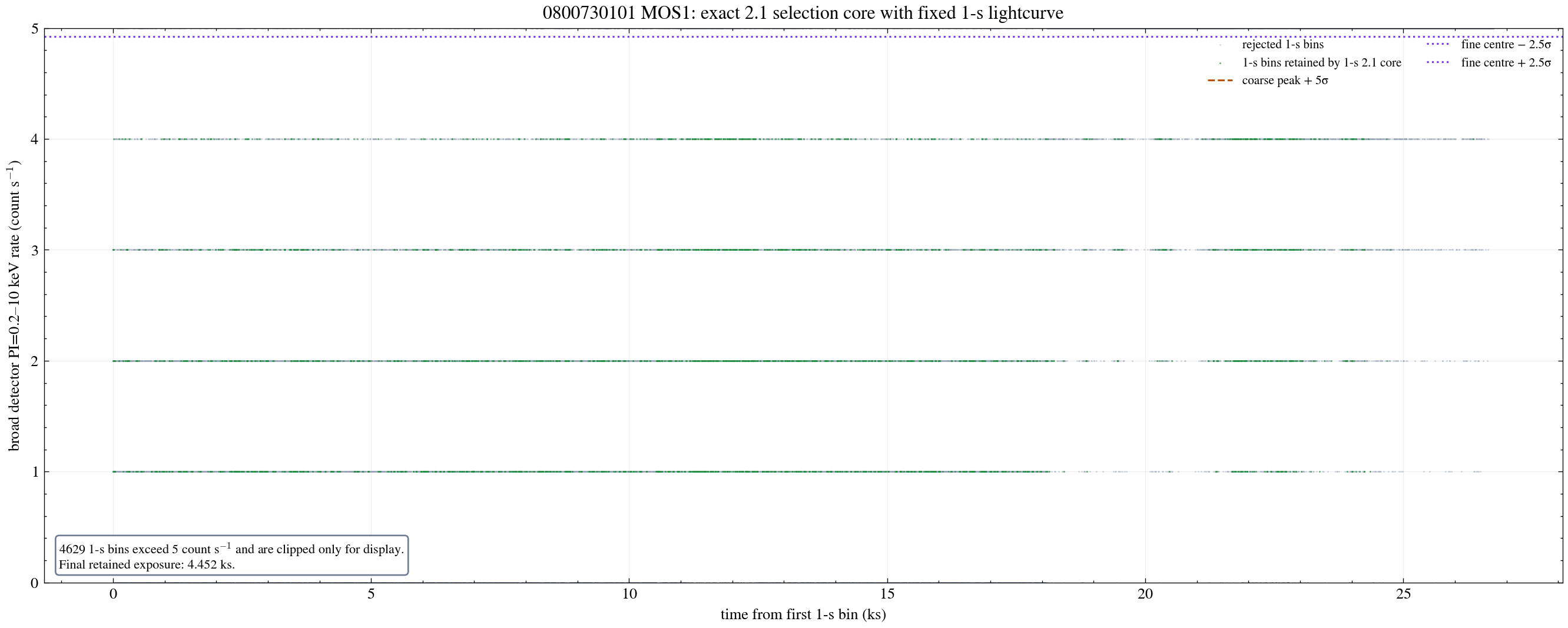
This uses 2.1.filter/mos1S001-ori.fits, keeping the reviewed espfilt.py selection logic and only changing timebin to 1 s; the run stops at the candidate-GTI stage and does not generate SAS/ESAS spectra or responses. The input is 84,865 broad-detector PI=0.2–10 keV events, 26.750 ks, mean 3.585 counts/s.
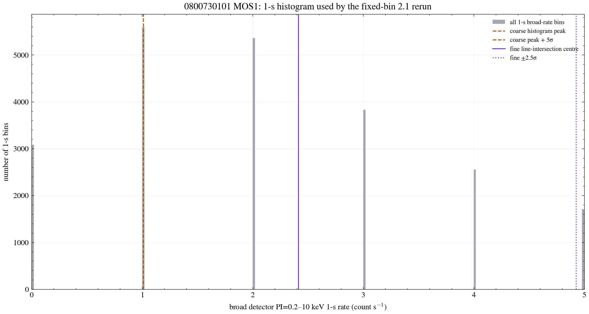
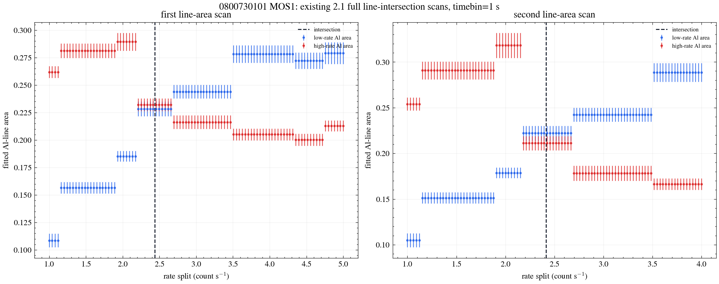
The conclusion is negative: the 1-s histogram's peak=1.01 counts/s, σ=1.005 counts/s is the mode of integer counts, not a stable background mean. The instrument-line "intersection"=2.413 counts/s falls between the staircase-like selection steps and cannot be treated as a physically resolved centre. The final GTI is only 4.452 ks / 1,181 segments, and its overlap with the historical 2.1 GTI is only 0.456 ks (Jaccard=0.0837). So 1 s can be kept for flare timing, but cannot directly replace the existing baseline/zero-neighbour/line-intersection estimator.
0800730101 MOS1: QDP51 re-run of the 2.1 strategy 2026-09-03 · isolated test arm
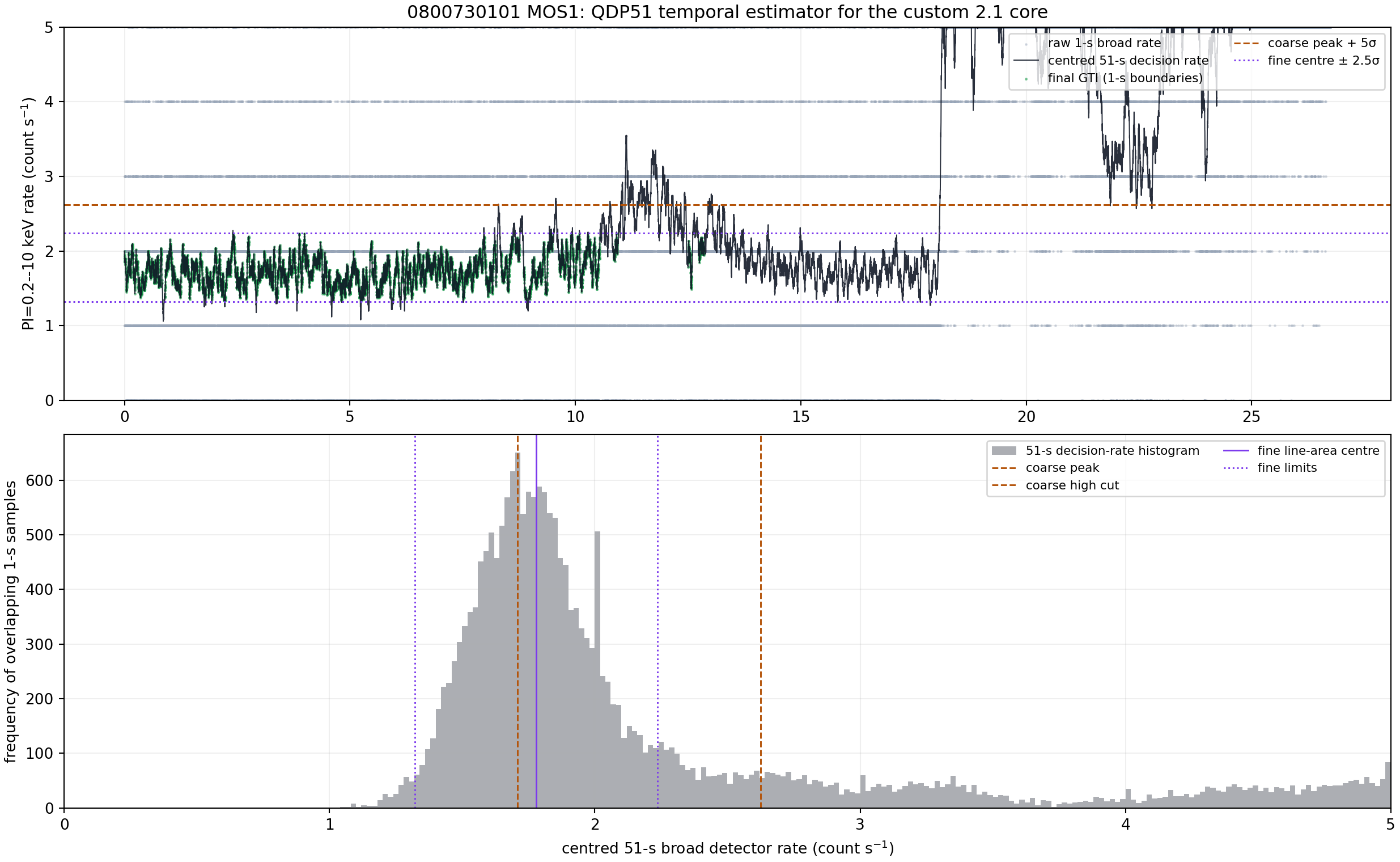
This time the 1-s discrete counts are not used directly for the baseline or line-intersection. First the raw broad-detector PI=0.2–10 keV events produce a 1-s rate, then a centred 51-s sliding window builds the histogram, Poisson threshold and two-round instrument-line area scan decision variables; the final GTI is still written from the original 1-s boundaries and re-filters the events. Adjacent 51-s continuous samples share 50 s, so the histogram's high frequency does not represent the same number of independent measurements.
| Product | Final GTI | clean events | output lightcurve |
|---|---|---|---|
Historical 2.1.filter | 1.455 ks / 11 segments | 3,665 | 100-s rate |
This run 2.1qdp51 | 9.861 ks / 41 segments | 20,586 | 60-s rate and ratec, 446 rows each |
Construction check passed: all 20,586 clean events lie inside the final GTI, ONTIME=9.861 ks, LIVETIME=9.628 ks. The figure shows, at top, the raw 1-s rate, the 51-s smoothed rate used for decisions, the finally retained 1-s bins, and the coarse/fine thresholds; below is the overlapping 51-s sample histogram at 0–5 counts/s.
Key boundary: this only proves the new screening product is readable and its event/GTI membership is self-consistent; it has not yet produced a matched 3B/4.background spectrum or XSherpa fit. It therefore cannot be read as "SP has decreased" or "sky background is more stable"; the next step must compare spectra directly with the same region, response and rebinning.