Figure-led tutorial · group meeting

Single-observation Pareto GTI:
line constraint and continuum invariant

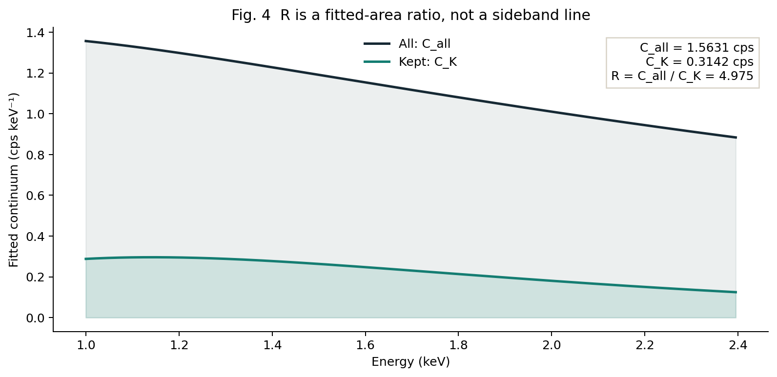
In one sentence: for one observation, find the Pareto frontier of retained live time $$T_K$$ and continuum reduction $R=C_\mathrm{all}/C_K$ subject to $L_\mathrm{all}=L_K$ .

Selection band2.5–8.0 keV

The FOV light curve constructs the GTI; CORNER is diagnostic only.

Fit band1.000–2.395 keV

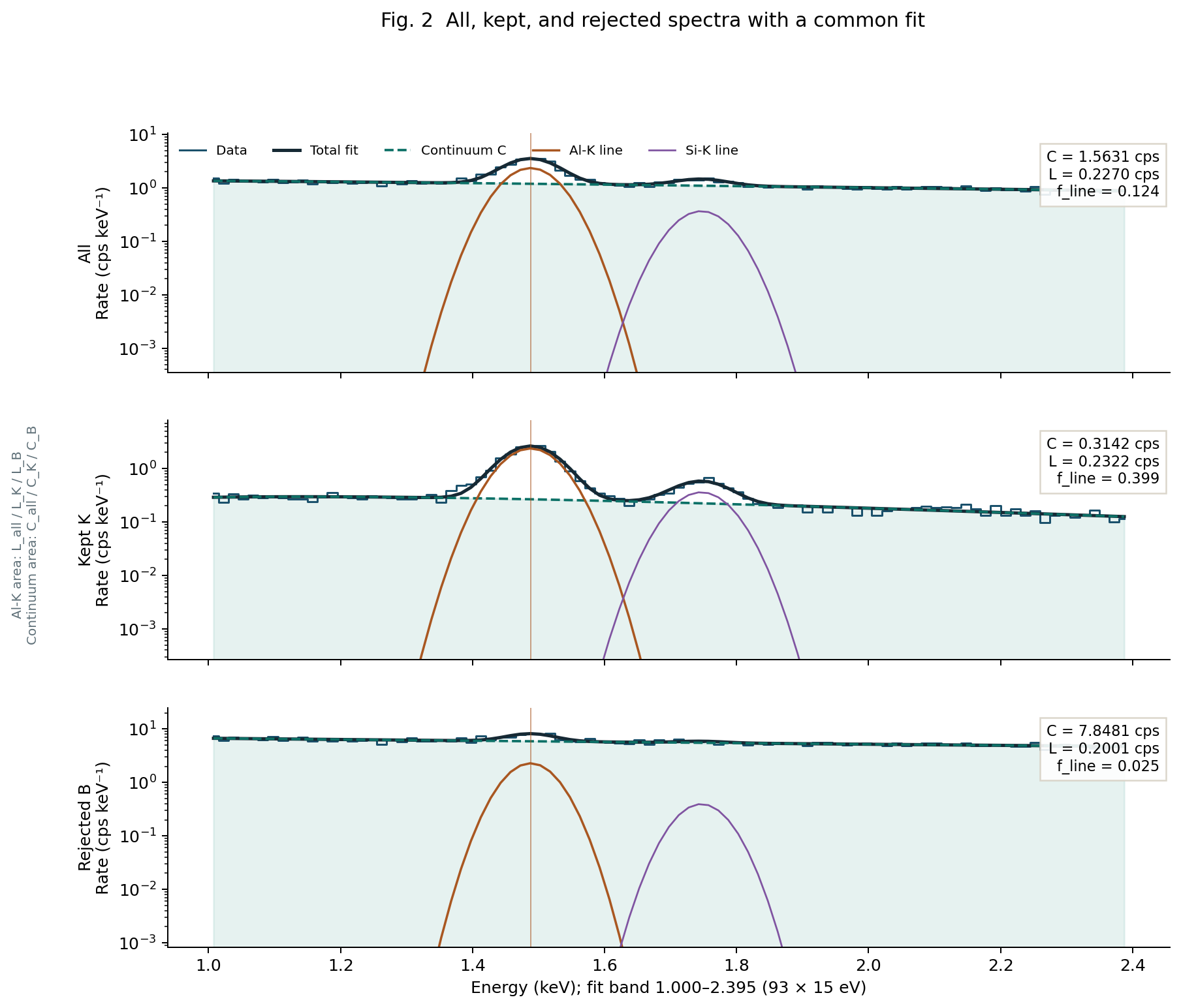
93 15 eV bins; Al-K=1.4879, Si-K=1.7466 keV.

ComparisonWithin one observation

$f_T=T_K/T_\mathrm{all}$ and $$R$$ ; averaging or ranking across observations is forbidden.

Part 1 · anatomy

1. First split one observation into all, kept, and rejected

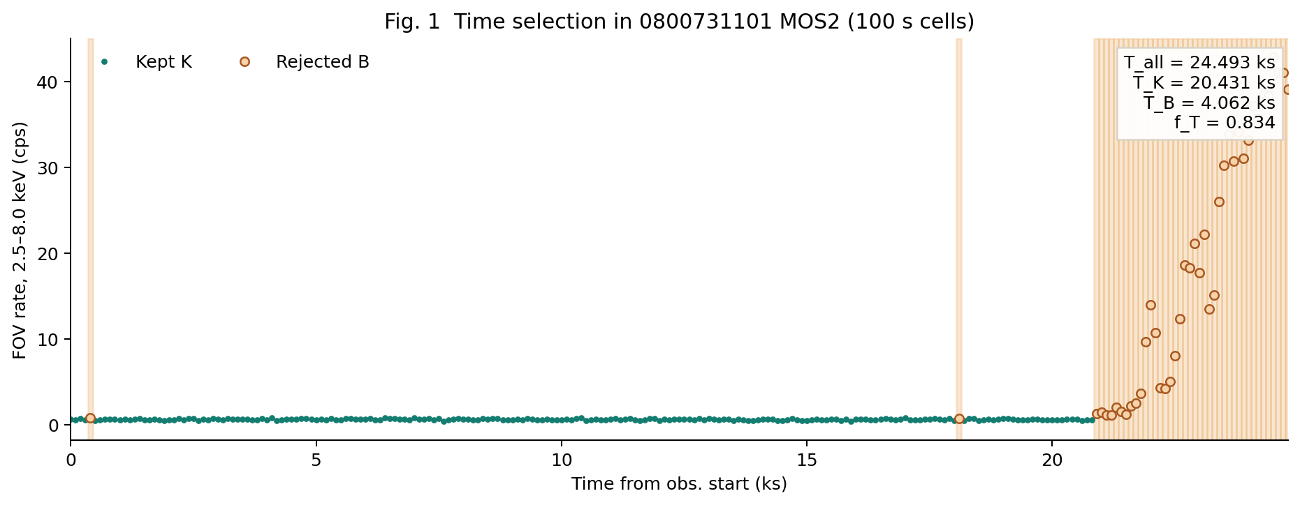
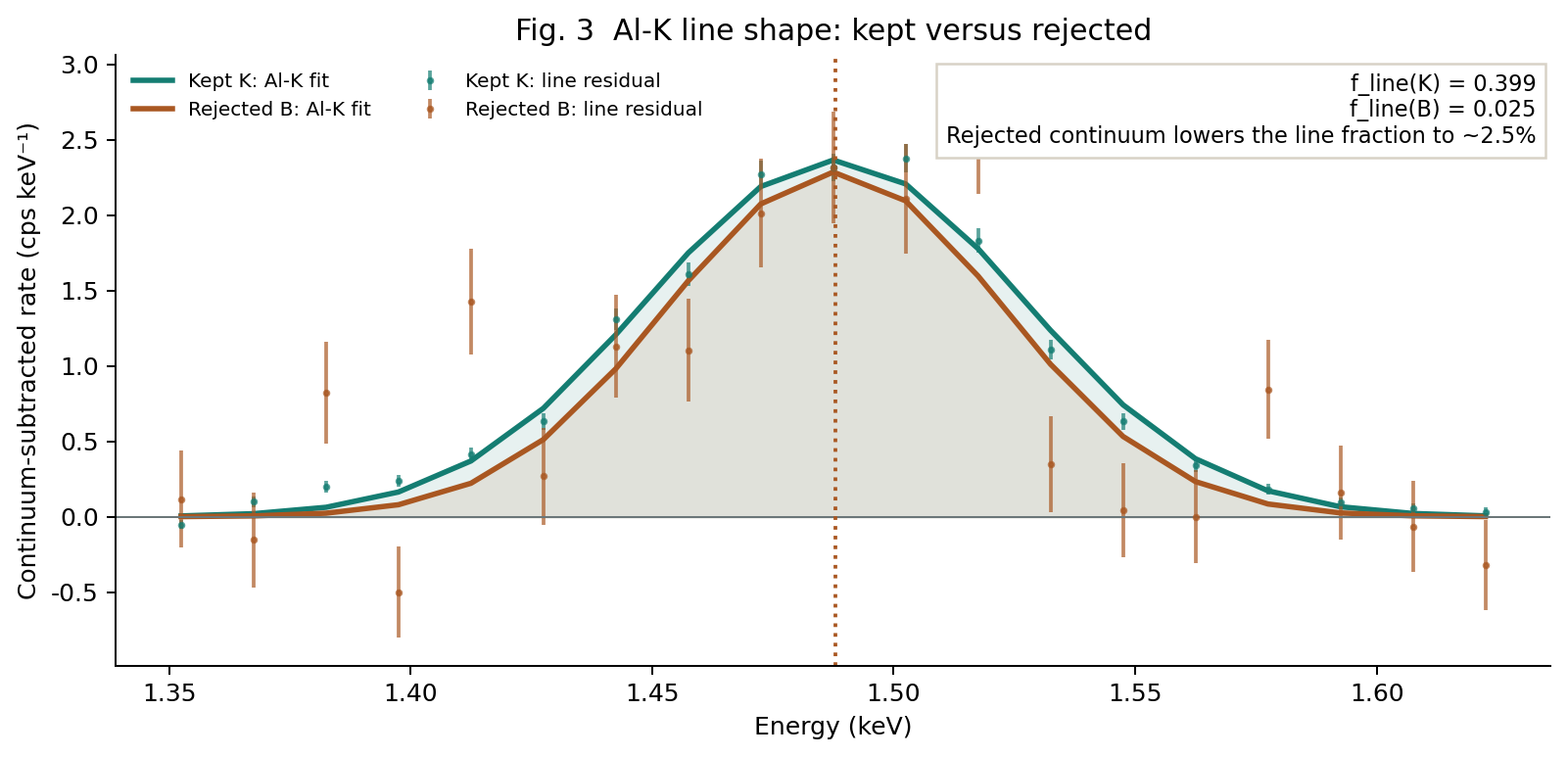
The next four figures use the strong-flare observation 0800731101 MOS2. Each 100 s cell gets its live time from the segment-by-segment sum of TIMEDEL × FRACEXP; containing events does not imply a full 100 s.

Live-time-corrected 2.5–8.0 keV FOV light curve for 0800731101 MOS2 in 100 s cells, showing kept and rejected cells — Fig. 1 Start with time: the terminal flare is assigned to B. The measured values are $T_\mathrm{all}=24.493$ ks, $$T_K=20.431$$ ks, and $$T_B=4.062$$ ks, giving $$f_T=0.834$$ . Shading marks K/B partitions accounted with measured live time, not event counts.

All, kept, and rejected 1.000–2.395 keV spectra and fit models for 0800731101 MOS2 — Fig. 2 This is the symbol map: the Al-K Gaussian areas are $L_\mathrm{all},L_K,L_B$ ; the green continuum areas over the 93-bin window are $C_\mathrm{all},C_K,C_B$ . All three use the same Cash fit: one log-parabola plus Al-K/Si-K Gaussians with fixed line centers.

Continuum-subtracted Al-K line for 0800731101 MOS2, comparing kept and rejected intervals — Fig. 3 Follow the same line, not a sideband: $f_\mathrm{line}=0.399$ for K and only 0.025 for B. The rejected continuum brightens, but the line itself does not; its relative noise grows. Thus $$L$$ must come from a curved spectral fit, not linear interpolation on either side of the line.

Fitted continuum areas for all and kept 0800731101 MOS2 data, with their R ratio — Fig. 4 $$R$$ is the ratio of two fitted continuum areas from one observation: $C_\mathrm{all}=1.5631$ cps and $$C_K=0.3142$$ cps, giving $$R=4.975$$ . It is neither sideband subtraction nor an absolute soft-proton flux.

Part 2 · constraint

2. The line that makes R meaningful also blocks score gaming

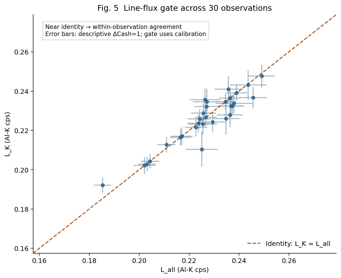
R(K)=\frac{C_\mathrm{all}}{C_K},\qquad L_\mathrm{all}=L_K,\qquad f_T=\frac{T_K}{T_\mathrm{all}}.

Maximizing $$R$$ means lowering the continuum while preserving the all-interval Al-K line only when the line-flux conservation gate holds. Since $L_K-L_\mathrm{all}=(1-f_T)(L_K-L_B)$ , more aggressive cuts make the gate more necessary and increase its testing power at the same time.

L_all versus L_K for 30 MOS2 observations with the identity line — Fig. 5 The all/kept Al-K fluxes for 30 observations lie around the identity line. The gate reference is **the same observation's** $L_\mathrm{all}$ , not a campaign mean; the across-observation Al-K value $\chi^2/\mathrm{dof}=339.41/29=11.70$ cannot rescue a candidate whose line is buried by its continuum.

R and line-gate trap for disjoint and overlapping selection bands in observations with no detectable variability — Fig. 6 · OVERLAP TRAP If the selection band overlaps the fit band, sampling follows noise in its own denominator: for 0800730201 the observed invalid-overlap point has $$R=1.078$$ , $z_\mathrm{null}=+6.86$ , and $$L_K/L_B=0.813$$ ; for 0800730401 they are $$R=1.073$$ , $z_\mathrm{null}=+5.96$ , and $$L_K/L_B=0.785$$ . The red configuration is diagnostic only: the formal program aborts on band overlap and assigns no gate verdict. The specification table also records independent invalid-gate diagnostics 0.8034/−4.6σ and 0.7680/−5.4σ; the two records differ by version, as documented in the delivery report.

Wording boundary

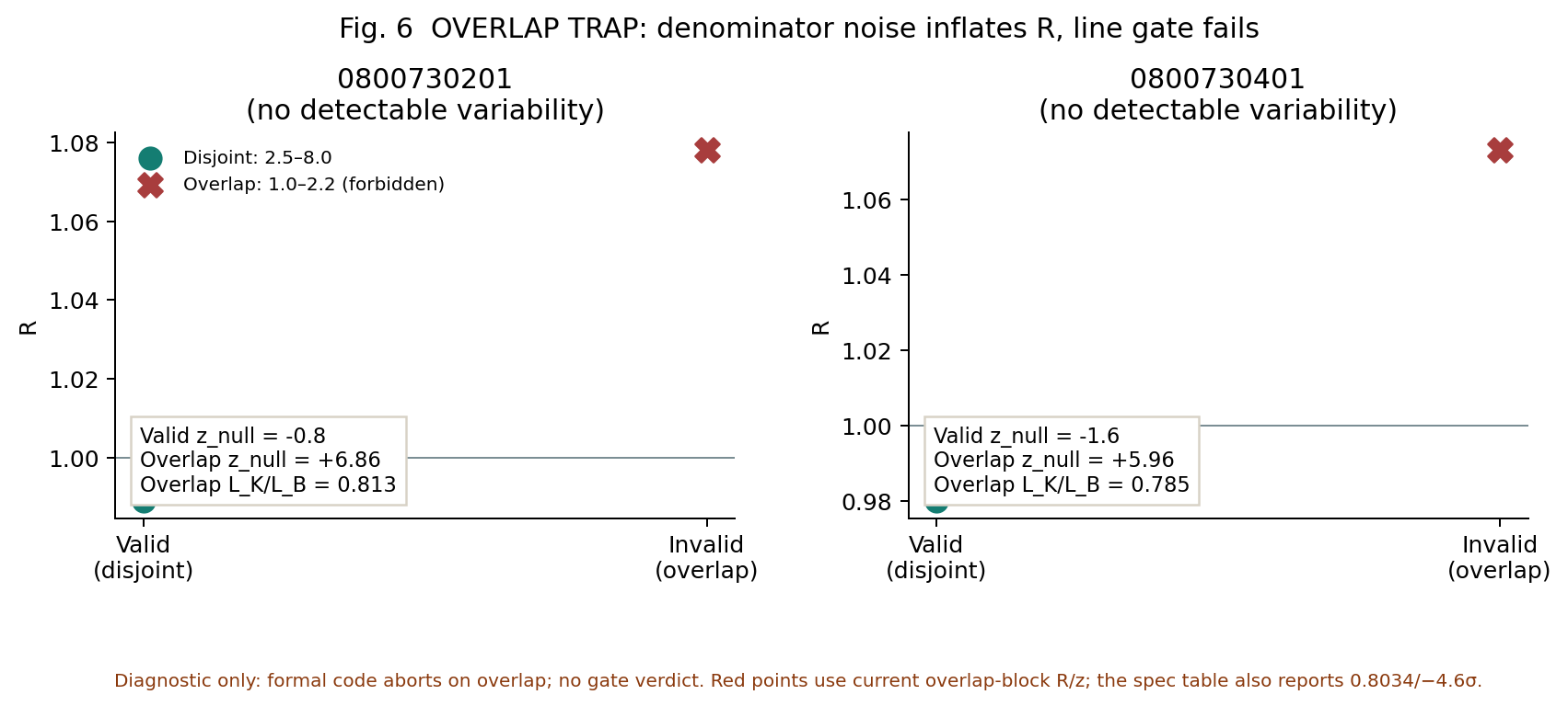
“No detectable variability” does not mean “no soft protons”: 0800730201 still has a small transient focused soft-proton signature, while steady soft protons remain by construction in $C_\mathrm{all}$ and $$C_K$$ , invisible to $$R$$ .

Part 3 · frontier

3. A curve is not a frontier: strategy structure must differ

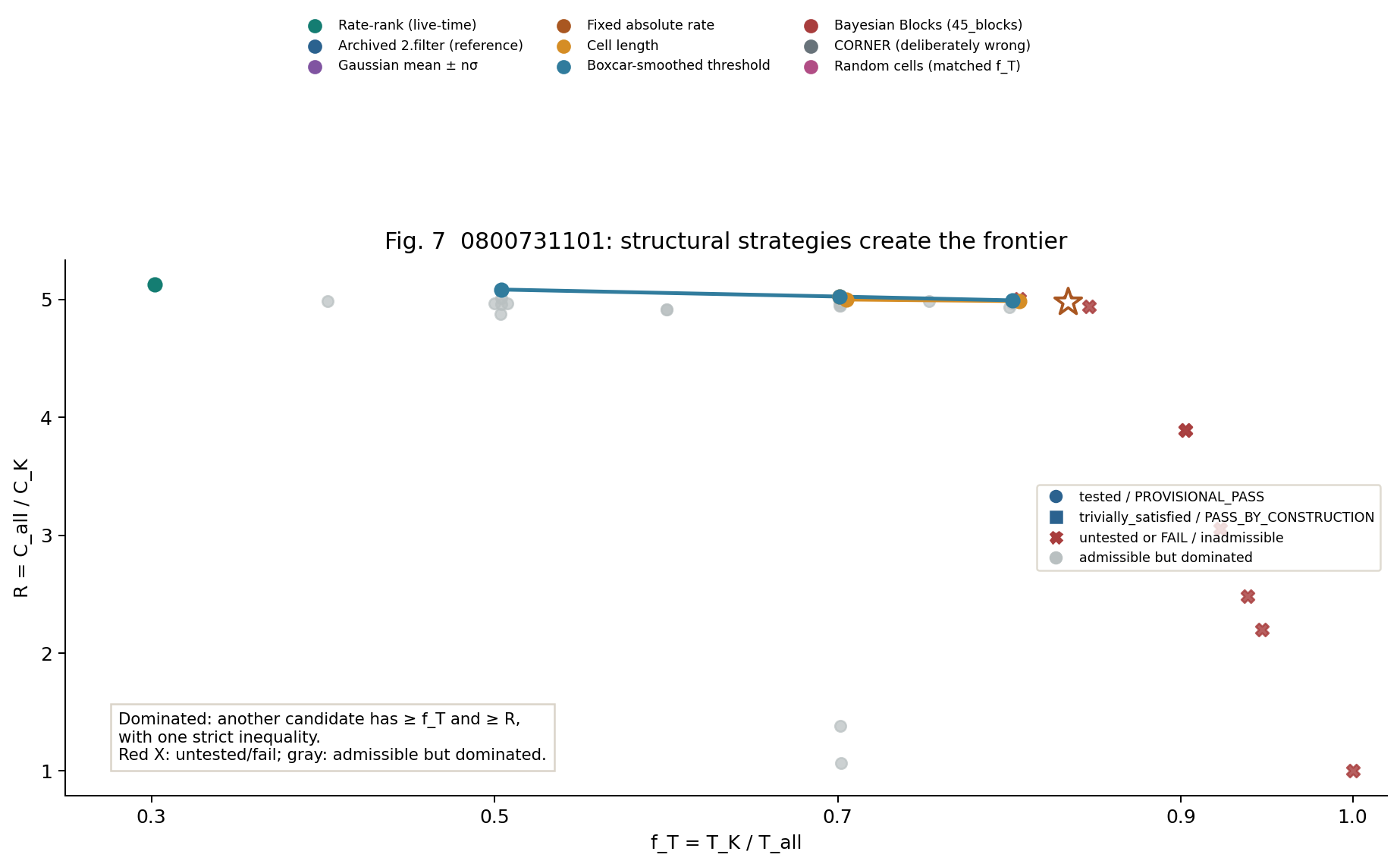
Changing only the retained fraction under one rate-rank rule usually produces a monotone curve, with no necessarily dominated point. This page therefore constructs 33 candidates on 0800731101 (25 new structured candidates), adding cell lengths, smoothing, histogram cuts, fixed-rate thresholds, Bayesian Blocks, CORNER, and a random baseline; every candidate refits K/B and carries a gate class and verdict.

Strategy family	Count	Definition
rate-rank (measured live time)	8	$f_T=0.30,\ldots,1.00$ ; existing rule.
Archived 2.filter (reference)	1	Star in the figure; not a new strategy family.
Gaussian mean ± nσ	3	$$n=1.5,2,3$$ ; keep cells within the histogram mean ± nσ.
Fixed absolute-rate threshold	3	Thresholds come from this observation's measured-rate quantiles and are not transferred across observations.
Different cell lengths	9	50/200/500 s, each at $$f_T=0.5,0.7,0.8$$ .
Boxcar-smoothed threshold	6	Smooth 5/11 original 100 s cells, each at three target fractions.
Bayesian Blocks	1	45 event-time blocks, retaining about 0.70 by block rate.
CORNER selection (deliberately wrong)	1	Rank by the corner curve; used only to show the wrong direction.
Random cells (matched $$f_T$$ )	1	Random-rate ranking to about 0.70; a dominated lower bound.

Structured Pareto frontier of f_T and R for multiple strategies on 0800731101 MOS2, showing gate markers, dominated points, and strategy families — Fig. 7 This is the tutorial's core: domination means another candidate has no lower $$f_T$$ and no lower $$R$$ , with at least one strict improvement. Circles/squares mark provisional passes that are tested / trivially_satisfied; red X marks untested or failed, inadmissible candidates; pale gray circles are admissible but dominated; colored lines are the current frontier; the star is the archived 2.filter reference. The reference itself has $\sigma_\mathrm{tot}=0.1213$ and is genuinely untested, so it is not a pass.

Candidate	$$f_T$$	$$T_K$ (ks)$	$$R$$	gate class / verdict
rate-rank 0.30	0.3021	7.399	5.126	tested / PROVISIONAL_PASS
cell 200 s, 0.70	0.7011	17.173	5.024	tested / PROVISIONAL_PASS
cell 200 s, 0.80	0.8059	19.739	4.985	tested / PROVISIONAL_PASS
cell 500 s, 0.70	0.7052	17.273	4.998	tested / PROVISIONAL_PASS
smooth 11 cells, 0.50	0.5038	12.341	5.083	tested / PROVISIONAL_PASS
smooth 11 cells, 0.70	0.7012	17.175	5.023	tested / PROVISIONAL_PASS
smooth 11 cells, 0.80	0.8020	19.644	4.991	tested / PROVISIONAL_PASS

The deliberately wrong CORNER strategy ( $$f_T=0.7014,R=1.383$$ ) and the random matched strategy ( $$f_T=0.7017,R=1.066$$ ) both lie below the frontier, as expected. They remain visible as wrong-choice and noise-floor gray points.

Rate-rank frontier shapes for three observations: no detectable variability, intermediate, and strong flare — Fig. 8 The same strategy family changes shape across observations: for 0800730201, $R=0.983\text{–}1.044$ varies only at the statistical-noise scale and operationally collapses to a point; the archived point is 1.564 for 0800730101 and 11.814 for strong-flare 0800732501. Height is set by each observation's own flare ceiling, so the three vertical axes are not a cross-observation ranking.

Part 4 · boundaries

4. Put the boundaries beside the conclusions

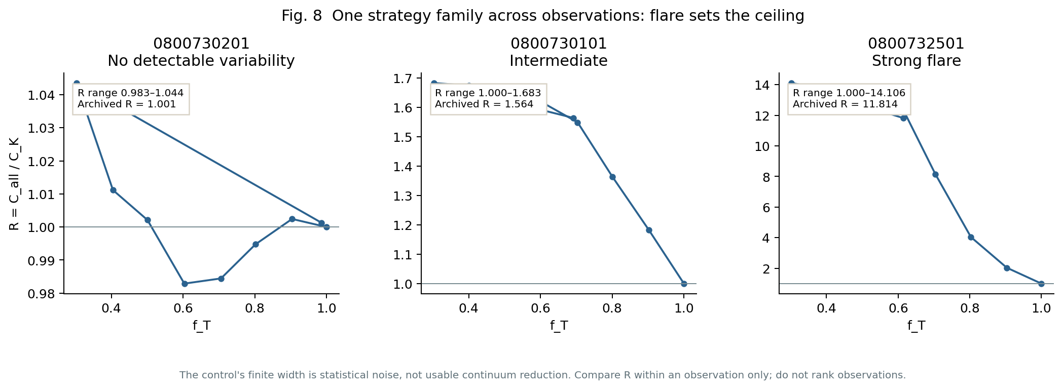
R is not comparable across observations

The ceiling of $$R$$ is set by how flared the observation happens to be, not by how good the strategy is. Therefore $$R$$ must never be averaged, ranked, or pooled across observations; frontiers are drawn per observation and only their shapes compare. It is not a soft-proton removal fraction.

Steady soft protons are invisible

A steady component raises the all and kept continua together, so $$R$$ can remain near 1; this framework therefore does not measure absolute SP counts.

R does not resolve bad CCDs or compact variables

Fault-injection receipts show that they can drive $$R$$ to about 4σ while the gate remains near 0. Independent CCD and spatial screening is required.

The gate verdict is provisional

The implementation records line–continuum coupling $s=-0.01284\pm0.00394$ and $s\lambda$ for every candidate, but the frozen adjudication does not apply the correction.

Two questions remain open

How should the direction and size of the line–continuum coupling correction ultimately be applied? Controlled injections give a negative slope, but the corrected full sample still shows about −2.2 to −2.5σ line loss, which could mean Al-K changes with particle flux or could indicate a second unmodeled system.
Al-K being stable in a linear-average sense does not mean that one observation lacks slow temporal structure; corner-particle rate must be tested as an independent probe.

Three takeaways

First, $$R$$ is a fixed-reference coordinate only within one observation. Second, the line both defines the gate for continuum reduction and prevents rate selection from turning noise into gain. Third, the frontier must come from structurally different strategies, and every point must carry a gate class and verdict.